Comparing Multiple Targets with Sample

When planning observations, it is common to ask: how does the required exposure time change with redshift? or how much data will I accumulate over a survey?

The slicersim.sample.Sample class lets you manage a collection of targets together and answer these questions efficiently.

import numpy as np
import matplotlib.pyplot as plt
import slicersim
from slicersim.sample import Sample

---

1. Build a sample of type Ia supernovae

Sample.from_sneia() creates a collection of LazuliSupernova objects at the given redshifts. The spectrograph field ("narrow" or "wide") is automatically selected based on the redshift: "narrow" up to z=0.8, "wide" beyond.

# Create a sample of 8 SN Ia spanning z=0.2 to z=1.4
redshifts = np.linspace(0.2, 1.4, 8)
sample = Sample.from_sneia(redshifts)
print(f"Sample has {sample.ntargets} targets")

Sample has 8 targets

You can access individual targets by index:

# Inspect one target
t0 = sample.get_target(0)
print(f"First target: z = {t0.get_properties('redshift'):.2f}, field = {t0.get_spectrograph_field()}")

First target: z = 0.20, field = ('narrow', {'spatial_shape': [58, 58], 'spatial_scale': 0.04})

---

2. Set up the sample to reach a given SNR

setup_to_snr() configures the detector readout mode of each target so that the requested mean SNR per resolution element is reached in the given wavelength window (here rest-frame).

%%time
# Aim for SNR=10 per resolution element in rest-frame 4000-7000 A
_ = sample.setup_to_snr(
    snr=10,
    per_resolution=True,
    lbda_range=[4000, 7000],
    frame="rest",
)

CPU times: user 2.11 s, sys: 742 ms, total: 2.86 s
Wall time: 2.86 s

---

3. Summary statistics

get_summary_stats() returns a DataFrame with the exposure time, the data volume and the detector readout configuration of each target.

stats = sample.get_summary_stats()
stats.index = np.round(redshifts, 2)
stats.index.name = "redshift"
stats

	volume	exptime	nramps	ngroups	nframes_per_group	ndrops
redshift
0.20	0.369099	124.52	1	11	4	0
0.37	0.771752	260.36	1	23	4	0
0.54	0.603980	407.52	1	18	8	0
0.71	0.838861	566.00	1	25	8	0
0.89	1.073742	724.48	1	32	8	0
1.06	1.308623	882.96	1	39	8	0
1.23	2.113929	1426.32	1	63	8	0
1.40	3.623879	2445.12	2	54	8	0

Notice how the readout mode (ngroups, nframes_per_group) and the number of ramps (nramps) increase with redshift, as the source gets fainter and longer exposures are needed.

---

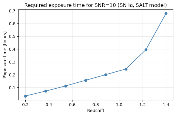
4. Exposure time vs. redshift

The cost of observing a SN Ia grows steeply with redshift.

exptimes_h = sample.get_exposure_time(units="hour")

fig, ax = plt.subplots(figsize=(6, 4))
ax.plot(redshifts, exptimes_h, "o-", color="steelblue")
ax.set_xlabel("Redshift")
ax.set_ylabel("Exposure time [hours]")
ax.set_title("Required exposure time for SNR=10 (SN Ia, SALT model)")
ax.grid(alpha=0.3)
plt.tight_layout()

---

5. Data volume vs. redshift

Higher-redshift targets require longer or more ramps, which increases the raw data volume of each observation.

data_volumes = sample.get_data_volume(units="GB")

fig, ax = plt.subplots(figsize=(6, 4))
ax.bar(redshifts, data_volumes, width=0.07, color="coral", edgecolor="k", linewidth=0.5)
ax.set_xlabel("Redshift")
ax.set_ylabel("Data volume per observation [GB]")
ax.set_title("Data volume per SN Ia observation")
ax.grid(axis="y", alpha=0.3)
plt.tight_layout()

---

6. Survey duration estimate

get_total_surveyduration() scales the exposure times of the sample to estimate how long a larger survey would take. It assumes that the survey targets follow the same distribution as the sample. By default, it assumes a survey of 8000 SN Ia and that 40% of the mission time is spent on it (fraction_survey=0.4).

# How many years would a 2000-target survey take with 40% of the mission time?
duration_yr = sample.get_total_surveyduration(sample_size=2000, fraction_survey=0.4, units="yr")
print(f"Estimated survey duration: {duration_yr:.2f} years")

Estimated survey duration: 0.14 years

---

7. Visualizing spectra across the sample

Loop over targets to retrieve and plot individual spectra.

fig, ax = plt.subplots(figsize=(8, 4))

cmap = plt.cm.viridis
for i, target in enumerate(sample.targets):
    lbda, flux, variance = target.get_spectrum(unit="flambda", incl_error=False)
    color = cmap(i / (sample.ntargets - 1))
    z = target.get_properties("redshift")
    ax.plot(lbda / 1e4, flux / flux.max(), lw=0.8, color=color, label=f"z={z:.2f}")

ax.set_xlabel("Wavelength [micron]")
ax.set_ylabel("Normalized flux")
ax.set_title("SN Ia spectra across redshift")
ax.legend(fontsize=7, ncol=2)
ax.set_xlim(0.4, 1.8)
plt.tight_layout()

As expected, the SN Ia spectral features shift to longer wavelengths at higher redshifts.